- Dataset
The dataset has 25 variables. There are 10 categorical features, 14 numerical features and 1 target variable. The aim of data analysis is to predict whether a customer will default next month in credit card payments. The critical aspect of the analysis is to accurately identify the potential defaulters. There is higher risk in misclassifying a potential defaulter as non-defaulter than in placing a non-defaulter in the defaulters’ list. Hence, the performance of a machine learning model will be determined by the overall accuracy as well as by the number of true positives vis-à-vis false negatives. Higher the ratio of true positives to false negatives, more robust the model. The model robustness is further tested in imbalanced datasets where the non-defaulters exceed the defaulters and the defaulters fall in the minority class.
2. Exploratory data analysis
The current dataset has 30000 rows and there are no null values. More than 75% of the use cases belong to the class of non-defaulters and the remaining are the defaulters as shown in Figure 1.
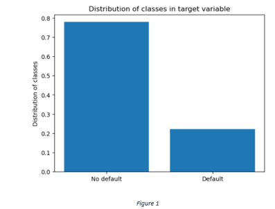
Figure 1
The range of age distribution is between 21 years and 80 years. The age distribution skewed towards left indicates greater proportion of clients falling in the younger age groups (Figure 2).
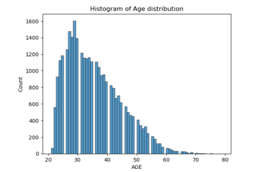
Figure 2
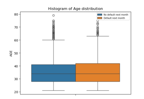
Figure 3
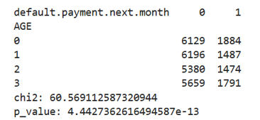
Although the box plots do not show any visible difference in the age distribution between defaulters and non-defaulters (Figure 3), a chi-square test performed on age (divided into 4 categories) shows significant difference in the distribution of defaulters and non-defaulters between different age groups.
A distribution of repayment status in different months in Figure 4 indicates that most of the customers pay on time and a relatively smaller proportion delays in repayments. Most of the repayment delays are between 1 to 2 months.
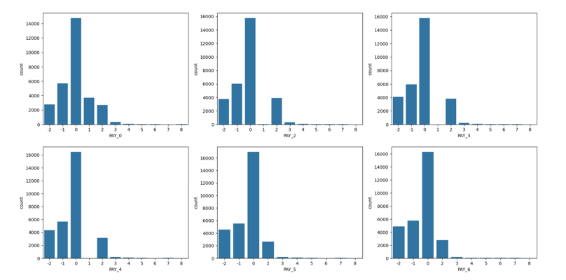
Figure 4
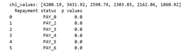
The repayment status is encoded into three categories; 0 for 0 or than 0 score, 1 for delay between 1 to 2 months and 2 for delay of more than 2 months. A distribution of target variable across different categories of repayment status scores in Figure 5 shows that more than 80% of customers making timely payments do not default. The percentage of customers delaying between 1 to 2 months is between 50% and 60%.
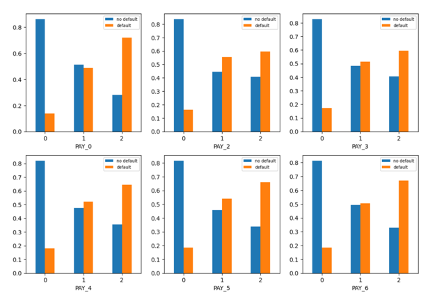
Figure 5
A chi-square test shows statistically significant difference in the distribution of defaulters and non-defaulters between different categories of repayment status, given 0.05 as the level of significance.
A distribution of target variable across different categories of ‘SEX’, ‘EDUCATION’, ‘MARRIAGE’, ‘AGE’ is shown in Figure 6.
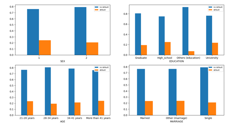
Figure 6
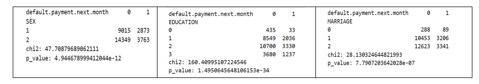
Similar chi-square tests for ‘MARRIAGE’ ‘EDUCATION’ and ‘SEX’ also show significant association between different categories of the categorical features and the target variable.
Table 1
3. Feature Engineering
Six engineered features are created:
Average payment across six months / Average bill across six months: The ratio of payments to the average bill amount indicates the outstanding balance. Higher the ratio, lower the outstanding balance, lower the probability of default.
Product of Repayment status of September and bill amount of September: Higher the score in repayment status and higher the outstanding bill amount, higher the product of repayment score and bill, higher the probability of default next month.
Average bill across months/ Limit balance: Higher the average bill vis-à-vis the limit balance, higher the probability of default.
Product of Repayment status of August and August bill amount: Higher the product of repayment score and bill, higher the probability of default next month.
Product of Repayment status of July and July bill amount: Higher the product of repayment score and bill, higher the probability of default next month.
Sum of Repayment status score of first three months: Higher the sum of repayment scores of first three months, higher the probability of default.
Sum of Repayment status score of last three months: Higher the sum of repayment scores of first three months, higher the probability of default.
The idea behind creating these engineered features is that the customers whose outstanding balance, average bill and delays in repayment are higher, are likely to have a higher probability of default.
Table 2 shows p-values of the t-tests conducted for some of the engineered features.
Table 2
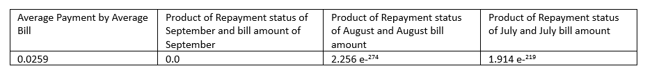
The t-tests show that at 0.05 level of significance there is a statistically significant association between each of the engineered features (table) and default next month. The t-test results show that the mean of values for each of the given features is higher for defaulters than for non-defaulters. The p-value less than 0.05 shows that the probability of observed difference in means between two classes by chance is very low.
4. Feature Encoding
The category ‘SEX’ is encoded using Label Encoder. The remaining categorical variables like ‘MARRIAGE’, ‘EDUCATION’ and ‘AGE’ are encoded using One Hot Encoder.
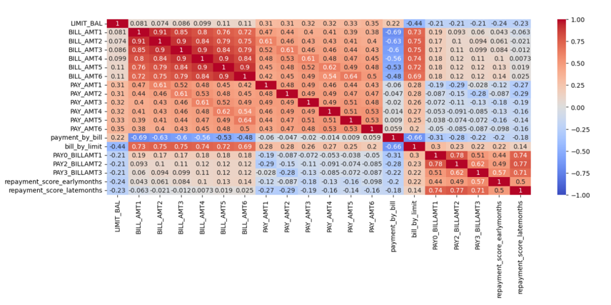
Figure 7
Figure 7 shows the correlation heat map of the quantitative variables. A correlation matrix among the numerical features shows high correlation among the outstanding bill amounts of different months. There is also a high correlation between bill by limit and the bill amounts and high correlation between the products of monthly repayment status scores and the monthly bill amounts. The average bill by limit is a clear representative of all the outstanding bills. Hence, the bill amounts of all the months except for the recent month of September can be filtered to remove redundancy in data features.
The following numerical features are further subjected to normalization in the range of 0 and 1: Repayment late scores, Repayment early scores, Limit balance, Bill amount of September, Payment amounts of all the six months, Average payment by average bill, Average bill by limit balance, Product of repayment score and bill of September, Product of repayment score and bill of August and Product of repayment score and bill of July.
One of the engineered features, ‘Average payment by average bill’ has many outliers. The outliers are removed by removing the values that are either lower than lower bound (Quartile1 – Inter quartile range*1.5) or higher than the higher bound (Quartile 3 + Inter quartile range*1.5). The distribution of the feature is shown in Figure 8.
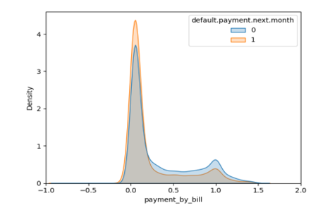
Figure 8
5. Model Building and Training
The data is split into 80% train and 20% test data.
Logistic Regression: The parameters are tuned using Grid Search CV. A stratified 5-fold cross validation is used for tuning inverse of regularization strength and l1 ratio. The selection of the best parameters is followed by training the model by using a combination of the chosen parameters and each of the three types of class imbalance handling techniques are used: Class weights, SMOTE-NC and ADASYN.
Class weights: It is a technique of modifying a model’s loss function by assigning higher weights to the errors incurred in misclassification of the minority class and lower weights to the error of the majority class. The aim is to let the model pay closer attention to the minority data points and reduce their probability of misclassification.
SMOTE-NC: Synthetic Minority Oversampling technique is an oversampling technique that synthesizes data points of the minority class and handles both categorical and numerical data. A variant of SMOTE, SMOTE-NC first applies SMOTE to synthesize samples of the numerical features and then uses the nearest neighbours of the synthetic samples to determine the values of categorical data.
ADASYN: Oversampling technique similar to SMOTE but adaptively generates synthetic samples of minority class based on the number of nearest neighbours of the majority class. The ideas is to synthesize more samples for harder to classify minority data points.
Figure 9 shows train and test data accuracies and F1 scores generated from Logistic Regression model and different class imbalance handling techniques.
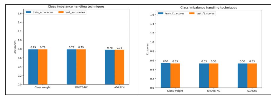
Figure 9
It is observed from Figure 9 that there is a negligible difference in both train and test data accuracies and F1 scores among different class imbalance handling techniques. Given the lower computational complexity, class weights will be chosen for Logistic Regression.
Decision Tree Classifier: The parameters used for hyper parameter tuning are criterion, maximum tree depth, minimum number of samples per split maximum number of features and minimum number of samples per leaf node. The class imbalance handling techniques used are: class weights, SMOTE-NC, ADASYN and under sampling method (Rus boost classifier). RUS boost classifier is a class imbalance handling technique that combines random under sampling of the majority class and boosting procedure of Ada boost.
Figure 10 shows train and test data accuracies and F1 scores from Decision Tree classifier model and different class imbalance handling techniques.
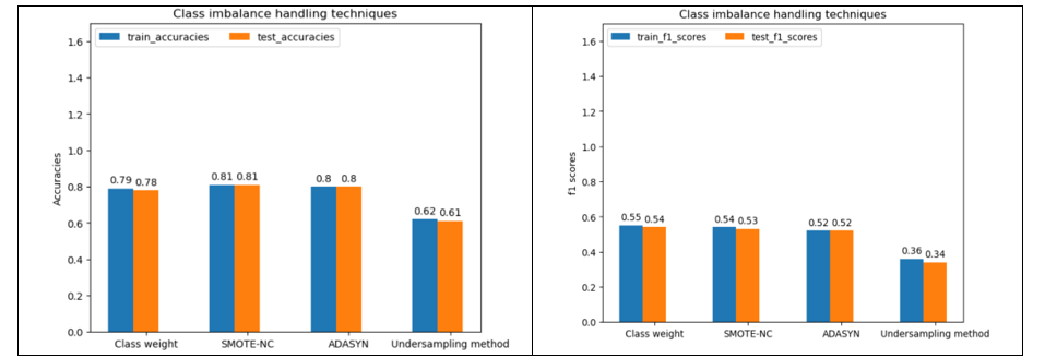
Figure 10
From Figure 10, SMOTE-NC offers better accuracies. However, F1 score is slightly higher for class weights. Overall high accuracy does not warrant better classification of minority class. F1 score, as a better indicator of model performance, is therefore used to select the class imbalance technique using Decision Tree classifier. Hence, class weight is selected.
Random Forest Classifier: After hyper parameter tuning, the class imbalance handling techniques are used to train the data. Figure 11 shows train and test data accuracies and F1 scores from Random Forest classifier model and different class imbalance handling techniques.
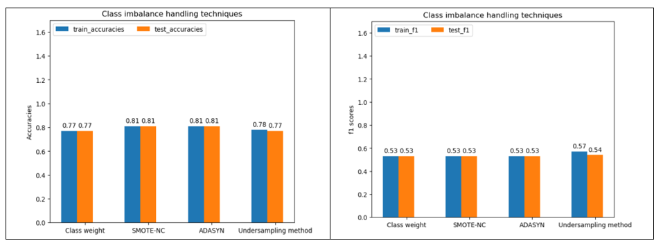
Figure 11
Under sampling method gives slightly higher F1 score for train and test data.
XG Boost classifier: The tuned hyper parameters are maximum depth, proportion of samples for training each base learner, proportion of features for training each decision tree, learning rate, number of estimators, gamma, minimum sum of instance weights needed in a child node. Figure 12 shows train and test data accuracies and F1 scores from training XG Boost classifier model and different class imbalance handling techniques.
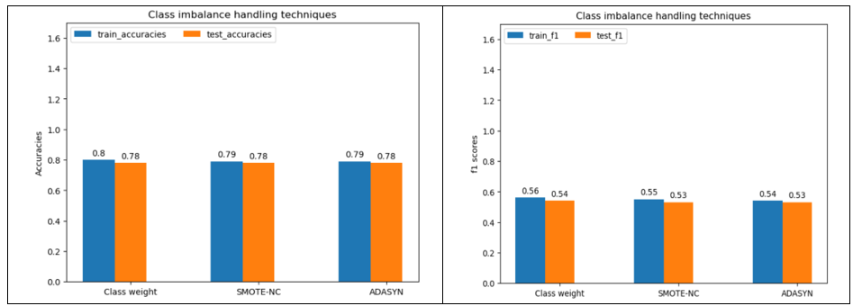
Figure 12
From Figure 12, class weights provide slightly better F1 score.
Light GBM classifier: Figure 13 shows train and test data accuracies and F1 scores from Light GBM classifier model and different class imbalance handling techniques.

Figure 13
From Figure 13, there is negligible difference in accuracies between class weights and SMOTE-NC. Class weight is selected due to slightly better F1 score.
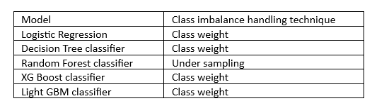
The best class imbalance handling technique selected for each model is shown in Table 3.
Table 3
6. Model comparison
The performance metrics (Accuracy, Recall, Precision and F1 score) of all the models for the train data are tabulated in Table 4 and for the test data in Table 5.
Table 4
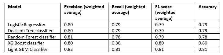
Table 5
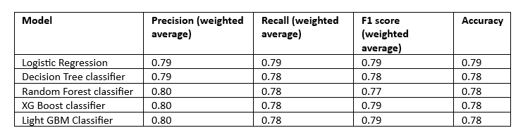
It is observed for the Tables that the performance metrics of all the models are nearly similar with Light GBM classifier having slightly higher values for the train data. Random Forest, XG Boost and Light GBM have the same weighted average precision. Overall, Light GBM and XG Boost have the same metric scores for the test data.
Figure 14 shows the Area Under the Curve (AUC) curve of all the models. The comparison of AUC curves is done separately for train and test data.
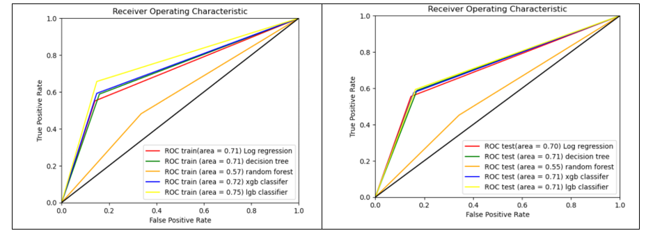
Figure 14
The Area Under Curve for the train data is the highest with Light GBM classifier. For the test data, Light GBM, XG Boost and Decision Tree classifiers have the same AUC score.
Precision and Recall curves are shown in Figure 15.
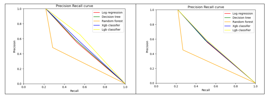
Figure 15
The Precision-Recall curves for test data are almost same for Light GBM, XG Boost, Decision Tree and Logistic Regression.
It is inferred from the observations that XG Boost or Light GBM exhibit similarity in performance on unknown data.
Model performance using untuned hyper parameters
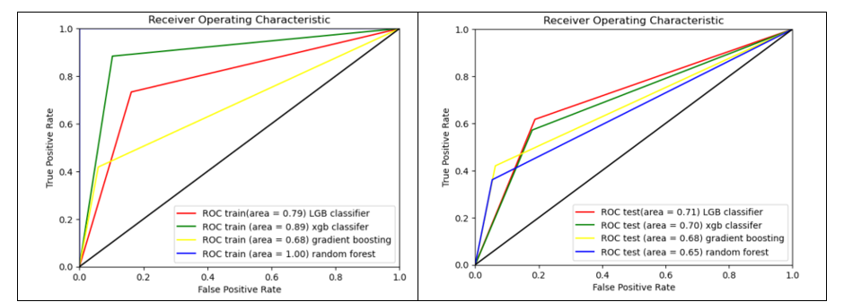
Figure 16
It is observed from Figure 16 that Light GBM classifier has an AUC score of 0.71 for both tuned and untuned parameters on test data. The performance metrics scores for the rest of the models are slightly lower than their tuned counterparts.
Light GBM is selected as the final model. The distribution of predictions generated by testing the trained Light GBM classifier on the test data and the actual distribution of likely defaults next month are shown in Figure 17.
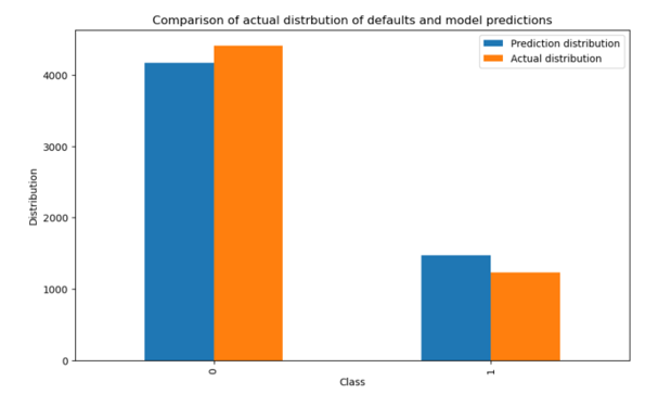
Figure 17
7. Feature importance and contribution in model predictions
The feature importance is calculated using SHAP values. SHAP value summary plot is shown in Figure 18.
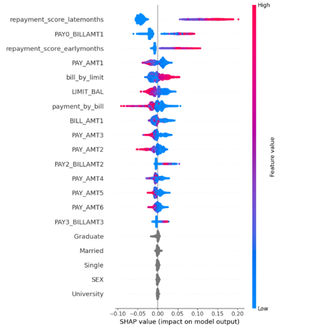
Figure 18
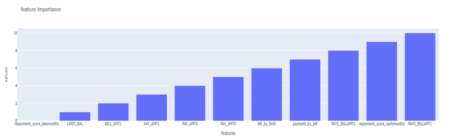
It is observed that some parameters like ‘Graduate’, ‘Married’, ‘Single’, ‘SEX’ and ‘University’ have very low SHAP values. A better picture of feature importance is shown in Figure 19.
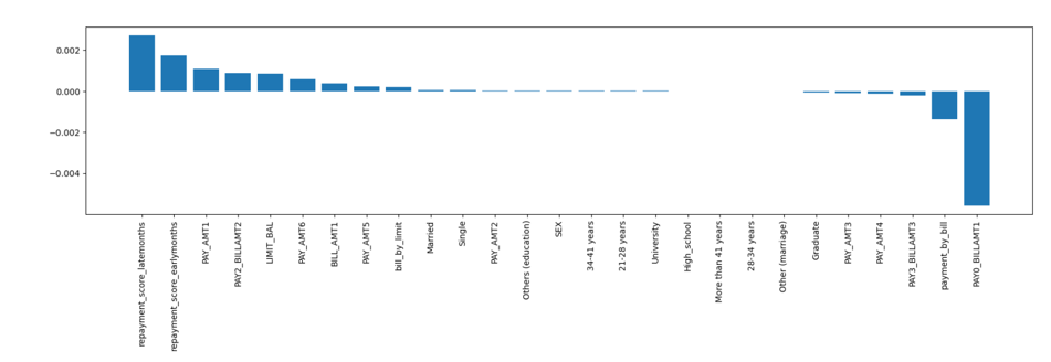
Figure 19
Based on the feature importance values, the selected features are: ‘repayment score late months’, ‘product of repayment status and bill of September’, ‘average payment by average bill’, ‘repayment score early months’, ‘Payment in September’, ‘product of repayment status and bill of August’, ‘limit balance’, ‘payment in April’, ‘September bill’, ‘payment in May’ and ‘average bill by limit balance’. The given variables are the most important in predicting default risk.
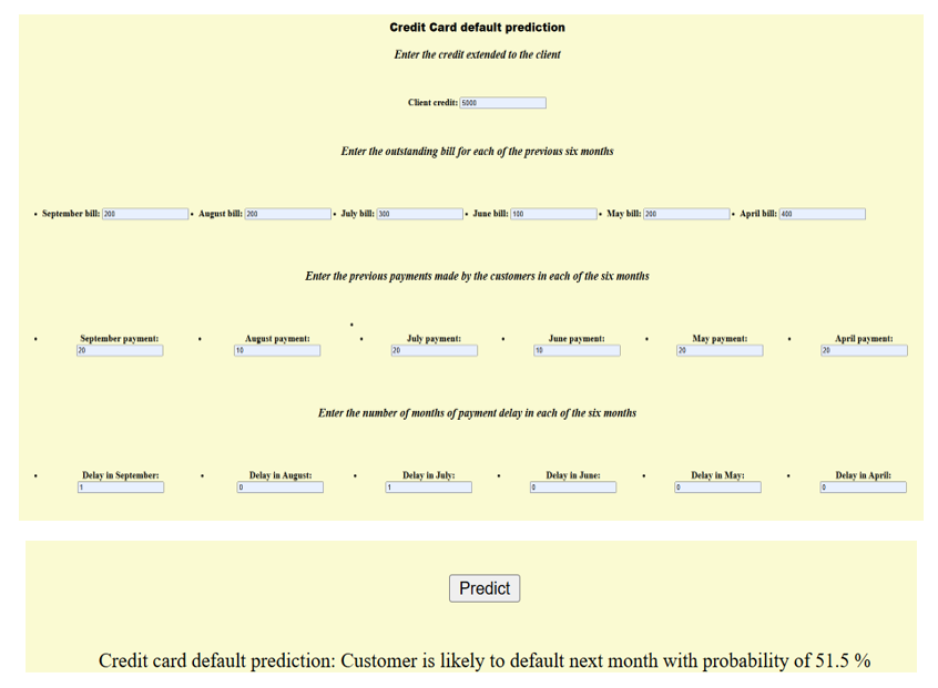
8. Web app Development
Creating web application: A web application framework named Flask was used for developing an interface that accepts customer bill and payment details and likely default next month with a certain probability. The trained model is saved as pickle file named ‘model.pkl’. Next, an application file named ‘cc_fraud.py’ is created in python. The file is the core of web application that responds to user requests based on the type of request. The Flask app is initialized and two functions are created. The first function is to display the content of HTML page of web app. The second function ‘POST’ is used to retrieve information from HTML file, feed the data to the trained model and send the prediction back to the HTML file to display the result. The third file is HTML file named ‘index.html’ stored in a ‘Templates’ folder. The HTML file consists of HTML code for creating input fields.
Deployment of web app: Following are the files created for web app deployment:
- model.pkl
- app.py
- Templates/index.html
Deployed app screen shots: