What to do if there are too few samples of a wine quality level?
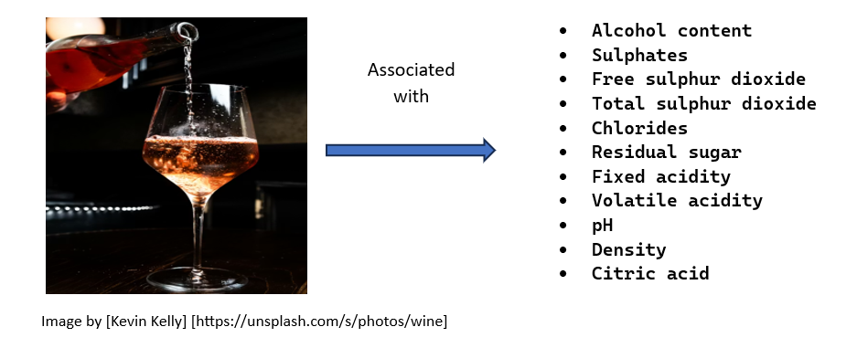
There were 11 indicators in this data set for identification of wine quality level. There was no information about the type of wine and the data set was limited to 1143 samples. The wine quality was represented in classes, where each class was associated with a particular level of wine quality. The wine quality levels were 3,4,5,6,7 and 8 where each succeeding level corresponded to higher quality wine. There were 6 samples of level 3 wine quality, 33 samples of level 4, 483 samples of level 5, 462 samples of level 6, 143 samples of level 7 and 16 samples of level 8.
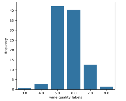
Figure 1: Percentage distribution of wine classes
For the given case, a step-by-step approach was adopted to tackle the challenge of a highly imbalanced data set.
Step by step approach:
- Exploratory data analysis
- Statistical tests
- Re-organisation of wine quality levels
- Model building and training
- Extract features strongly associated with wine quality
Exploratory data analysis
Univariate analysis
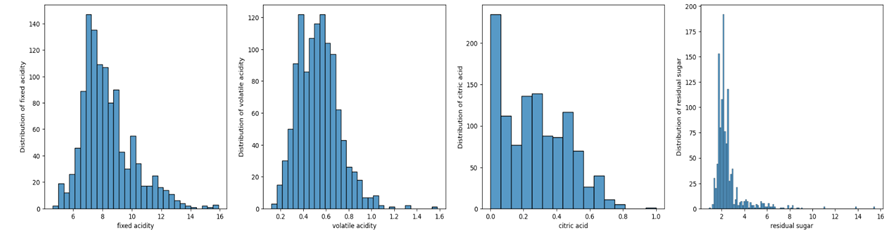
Figure 2: Histograms of fixed acidity, volatile acidity, citric acid and residual sugar
50% of fixed acidity was more than 8, with outliers in the range 12 to 16. 75% of volatile acidity was less than 0.6 and 75% of citric acid was below 0.4 in a range from 0 to 1. The distribution of residual sugar was highly skewed, with 75% less than 2.6 in the range between 1 and 16.
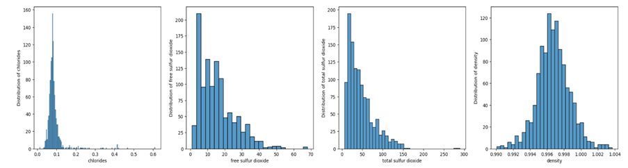
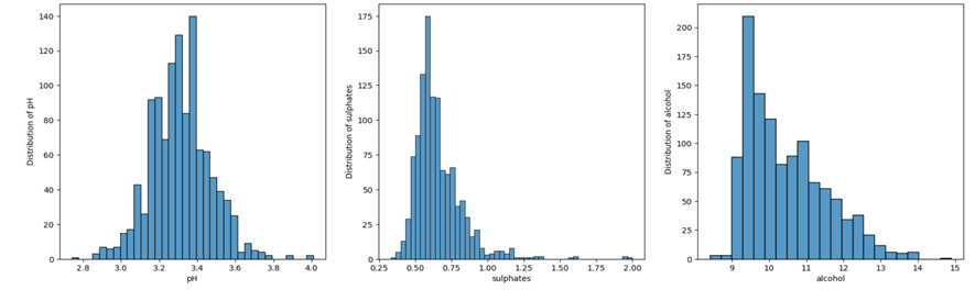
Figure 3
The Chlorides distribution was skewed with majority of the samples below 0.09. The outliers in chlorides were in the range beyond 0.11 to 0.6. Free sulphur dioxide ranged mostly between 1 and 40 with outliers extending from 40 to 70. Total SO2 was in the range 1 and 125 with outliers extending to 300. Density distribution approximated normal distribution with mean and median around 0.996. Most of the samples had pH in the range 2 and 3.8. Sulphates ranged between 0.25 and 1 with some outliers extending beyond 1 to 2. The mean and median of alcohol indicate that the distribution was right skewed, indicating most of the values of alcohol level fell in the lower range.
Bivariate analysis
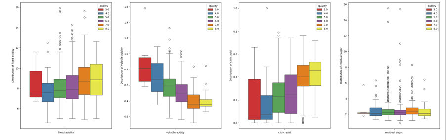
Figure 4
It is observed from Figure 4 that there was an overlap in the range of fixed acidity values across different levels of wine quality, with slight variation in the range of values. For instance, fixed acidity ranged between 4 and 10 for wine quality level 4 and between 6.5 and 11.5 for wine quality level 5. The median increased slightly as the wine quality level improved. From the observations, it was difficult to infer if the wine quality improves with improvement in fixed acidity.
Wine quality levels improved as volatile acidity reduces. For instance, 50% of volatile acidity of wine level 3 ranged between 0.65 and 0.95. 50% of volatile acidity of wine quality level 5 ranged between 0.5 and 0.65. 50% of acidity of wine level 7 further reduced to a range between 0.3 to 0.5. Similarly, wine quality levels improved with the improvement in citric acid levels, especially between wine level 4 and wine level 7. There appeared to be little difference in the distribution of residual sugar across wine quality levels, necessitating further investigation.
Figure 5
It was difficult to derive inference about the relationship between chlorides and wine quality, given a highly imbalanced dataset with very few samples of very low and very high-quality wine. Similarly, the association between wine quality and free SO2 and couldn’t be elicited from the boxplots. For instance, median of free sulphur dioxide was below 10 both for very high and very low wine levels but there was little variation in free SO2 median for levels ranging between 4 and 7. Similarly, at 50th percentile, SO2 level increased for wine level from 3 to 5 and decreased for higher quality of wine levels. It was apparent that moderate levels of free SO2 are needed for high levels of wine quality. An additional amount or insufficient amount of free SO2 may degrade the wine quality. There were overlap zones in density with slight decrease in median as wine level improved.
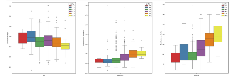
Figure 6
Lower the pH, better the wine quality. As seen from Figure 6, interquartile range (IQR) for wine quality level 3 ranged between 3.25 and 3.45. The IQR for wine quality level 8 was between 3.15 and 3.25. Sulphates are likely to have strong association with wine quality levels, given the quality showing significant improvement as the distribution range shifted from 0.375 – 0.675 to 0.675 – 0.875. 50% of alcohol in wine level 3 ranged between 9 and 10 and in wine level 7 ranged between 10.5 and 12.
Correlation Heat map
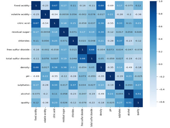
Figure 7
It is observed from Figure 7 that most of the feature pairs were weakly correlated. Fixed acidity was strongly correlated with density, citric acid and pH. Free sulphur dioxide, pH and residual sugar were weakly correlated with wine quality. The statistical tests showed statistically significant difference in total SO2 distribution between wine quality levels, while free SO2 did not show a significant difference. For the given data, the total SO2, appeared to be more important than stable free SO2 levels. The features with the lowest correlation with wine quality level were residual sugar, pH and free sulphur dioxide. Residual sugar also had weak correlation with other features, indicating that the association of residual sugar with wine quality was not strongly influenced by other intervening factors.
It is observed from Figure 7 that wine quality was more strongly correlated with alcohol and volatile acidity than with other parameters. A positive correlation of 0.48 between alcohol and wine quality indicated that higher alcohol content corresponded to better wine quality. Similarly, a negative correlation of -0.41 between volatile acidity and wine quality indicates that wine quality improved at lower levels of volatile acidity.
Statistical tests
Statistical significance of the relationship between each feature and wine quality
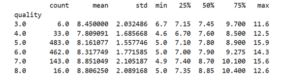
Table 1: Left side is statistical summary of residual sugar and right side is statistical summary of chlorides
The differences in means and median of residual sugar among different wine quality levels appeared negligible, suggesting that residual sugar by itself may not be a significant component influencing wine quality. The mean of chlorides decreased as the wine quality improved. Similar pattern was observed at 50th percentile, 75th percentile and the maximum level of chlorides, indicating consistency in the pattern of relationship between chlorides and wine quality.
Table 2: Left side is statistical summary of fixed acidity
The average fixed acidity increased as wine quality improved. However, the increase was not monotonic at different percentiles.
Table 3: Left side is statistical summary of free SO2 and right side is statistical summary of total SO2
The sample statistics of free SO2 depicted a distribution where the mean, median and other percentiles followed a curve of monotonic increase followed by monotonic decrease. The distribution shows that free SO2 was lower for low quality wines, improved as the quality improved and plummeted for high quality wines. A similar pattern is observed in total SO2 distribution as well. The sample statistics indicate that moderate levels of total SO2 are required for high quality wines.
Table 4: Left side is statistical summary of density and right side is statistical summary of pH
While the observed difference in density distribution is negligible, the density means and medians and percentiles plummeted as the wine quality improved. Further tests were conducted to establish statistical significance of density vis-à-vis quality levels. The pH means decreased with the improvement in wine quality. However, there was little difference in the observed distribution of pH levels across wine classes.
Testing the statistical significance of relationship between each feature and wine quality
Null Hypothesis: There is no difference in means of each feature among different wine quality levels.
Alternate hypothesis: There is significant difference in means of features among wine quality levels.
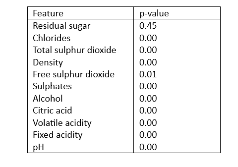
The imbalanced distribution of wine classes, fewer than 30 samples in some classes and non-normal distribution of features rendered the samples ineligible for a standard t-test. Hence, Krusal Wallis test was used to test if the difference in means across different wine categories was statistically significant for each feature. A significance level of 0.05 was assumed and the probability values (p-values) for each feature, as computed from the Krusal Wallis test, are shown in Table 5. The p-value is the probability that the observed differences in means, given the null hypothesis to be true, has occurred by chance.
Table 5
Results of post hoc tests
Table 6
As observed from post hoc test results in Table 6, at a significance level of 0.05, the difference in residual sugar between different pairs of wine quality was not statistically significant. There was also consistency in p-values for all other features between wine quality levels 7 and 8, indicating that the two wine levels could be combined to create a single indicator of high-quality wine. On the other hand, low quality wine levels did not show significant differences from other wine levels in terms of free sulphur dioxide, chlorides, pH, total sulphur dioxide, density, fixed acidity and citric acid. This could be due to very few samples resulting in underrepresentation of low-quality wine levels.
In terms of citric acid, volatile acidity, chlorides, alcohol and sulphates, wine quality at level 6 showed statistically significant difference from other (at least from 5, 7 and 8) wine quality levels. From the given test results, the wine levels with similar characteristics were combined to represent one category of wines. Three wine levels were derived from the results: wine levels 3-5 were combined to represent low quality wine (the differences among them were statistically insignificant) wine 6 was represented as medium quality wine (significantly low p-values (<0.05) with other wine levels) wine 7 and 8 were combined to represent high quality wine (consistently higher p-values (>0.05) indicating statistically insignificant differences in wine parameters).
Re-organisation of wine quality levels
From the post hoc analysis of Table 6, the differences in feature means, between each pair of wine levels 3,4 and 5, were statistically insignificant. There was statistically significant difference between wine level 6 and 7 for features like chlorides, density, sulphates, alcohol, citric acid, volatile acidity and fixed acidity. The wine level was also significantly different from wine level 5 for features like chlorides, density, sulphates, alcohol and volatile acidity. The wine levels 7 and 8 were similar.
- Wine level 7 and 8 were combined into one category ‘high quality wine’. (Sample size: 159)
- Wine levels 3,4 and 5 were combined into one category ‘low quality wine’. (Sample size: 522)
- Wine level 6 was identified as ‘moderate quality’ wine. (Sample size: 462)
The re-organisation of labelled responses refined the sample distribution across wine classes through an optimisation of wine quality levels.
Note: The results of the statistical tests may vary with the sample size and therefore, cannot be generalised for the entire population. A more pronounced representation of very low and very high -quality wine can alter the significance of relationship between wine quality and each feature.
Post hoc tests after altering classification of wine quality levels
Table 7
It was observed from Table 7 that at the significance level of 0.05, the difference in means between each pair of classes is statistically significant except for features like residual sugar, free sulphur dioxide and pH.
Based on the results of Post hoc tests, correlation Heat map and Scatter plots, residual sugar, pH and sulphur dioxide were the least important features associated with wine quality levels. Hence, Residual sugar, pH and free Sulphur dioxide were removed from the analysis.
Model building and training
XG Boosting Classifier
XG Boosting Classifier was used to address the challenge of model overfitting. The classification algorithm was applied in two ways:
- Untuned model
- Hyper parameter tuning + Class imbalance handling using SMOTE
For the tuned model, Grid Search Cross Validation was used to identify the best combination of hyper parameters based on F1-macro values. F1-macro was used for parameter selection, as it is a multi-class classification where all the classes are treated equally. To handle class imbalance, SMOTE was used. SMOTE technique synthesizes minority class samples and mitigates the model bias towards the majority class. The trained model was applied to predict the probabilities of wine classes and the threshold, for class selection, was set at 0.4.
Figure 8 shows confusion matrices of tuned model and untuned model applied on train data.
Figure 8: Left side is for Untuned model and right side is for tuned model on train data
Figure 9 shows the confusion matrices of tuned model and untuned model applied on test data.
Figure 9: Left side is for Untuned model and right side is for tuned model on test data
The trained model predicted the class labels at 100 % accuracy on train data. However, the model performance deteriorated when tested on the unknown data. Both the tuned and untuned models delivered similar performance on train data, indicating that XG Boosting Classifier is a powerful ensemble technique that can capture the variations in train data even without the need to tune the hyperparameters. Hence, the model performance was tested by evaluating its ability to capture variations on unknown data. From Figure 9, the untuned model predicted 74% of label ‘0’, 65% of label ‘1’ and 62% of label ‘2’. On the other hand, tuned model predicts 74% of label ‘0’, 65% of label ‘1’ and 66% of label ‘2’.
Other performance metrics are shown in Table 8.
Table 8
| Performance Metrics | Train data (Untuned model) | Train data (Tuned model) | Test data (Untuned model) | Test data (Tuned model) |
| Accuracy | 1.0 | 0.97 | 0.69 | 0.69 |
| Precision | 1.0 | 0.97 | 0.69 | 0.67 |
| Recall | 1.0 | 0.97 | 0.67 | 0.68 |
| F1 macro score | 1.0 | 0.97 | 0.68 | 0.68 |
It is observed from Table 8 that the model performance deteriorated on test data and the untuned XG Boosting Classifier performed slightly better than the tuned model.
Balanced Random Forest Classifier
The ensemble technique was used to handle class imbalance. The class imbalance was further addressed by applying a combination of SMOTE and hyperparameter tuning. Figure 10 shows the confusion matrices of tuned model and untuned model applied on train data.
Figure 10: Left side is for Untuned model and right side is for tuned model on train data
Figure 11 shows the confusion matrix of tuned model and untuned model applied on test data.
Figure 11: Left side is for Untuned model and right side is for tuned model on test data
Other performance metrics are shown in Table 9.
Table 9
| Performance Metrics | Train data (Untuned model) | Train data (Tuned model) | Test data (Untuned model) | Test data (Tuned model) |
| Accuracy | 0.86 | 0.77 | 0.66 | 0.63 |
| Precision | 0.83 | 0.74 | 0.62 | 0.59 |
| Recall | 0.89 | 0.79 | 0.67 | 0.62 |
| F1 macro score | 0.85 | 0.75 | 0.64 | 0.60 |
It is observed that the untuned Balanced RF performed better than the tuned Balanced RF model both for train and test data.
Model comparison
The performance metrics were compared between the untuned models of XG Boosting and Balanced Random Forest Classifiers in Table 10 and Figure 12.
Table 10
| Performance Metrics | Balanced RF Classifier (train) | XG Boosting Classifier (train) | Balanced RF Classifier (test) | XG Boosting Classifier (test) |
| Accuracy | 0.86 | 1.0 | 0.66 | 0.69 |
| Precision | 0.83 | 1.0 | 0.62 | 0.69 |
| Recall | 0.89 | 1.0 | 0.67 | 0.67 |
| F1 macro score | 0.85 | 1.0 | 0.64 | 0.68 |
Figure 12: Left side is on train data and right side is on test data
It is observed that XG Boosting classifier performed better than Balanced RF Classifier. From Figure 12, it is observed that the area under PR curve, in predicting Class 1 and Class 2 wine levels, was higher in XGB than in Balanced RF Classifier.
It was inferred from Figures 8,9,19,11 and 12 and Tables 8,9 and 10 that untuned XG Boosting Classifier delivered superior performance than other trained models.
Extract features strongly associated with wine quality
The untuned XG Boosting Classifier is further applied on train data to extract the most important features associated with wine quality, as shown in Figure 13, 14 and 15.
Figure 13: Feature importance for low quality wine
Figure 14: Feature importance for moderate quality wine
Figure 15: Feature importance for high quality wine
It is observed from Figures 13, 14 and 15 that the most important features affecting wine quality were alcohol and sulphates. The importance of other features differs for different wine quality levels. For instance, volatile acidity and chlorides were important for low quality wine, apart from alcohol and sulphates. For moderate wine quality, the other important were total sulphur dioxide and citric acid. For high quality wine, the other important were volatile acidity and citric acid.
Hence, the important features were alcohol, sulphates, volatile acidity, citric acid and total sulphur dioxide. This is also evident from correlation heat map as shown in Figure 7 and correlation with wine quality tabulated in Table 11.
Table 11
| Alcohol | 0.52 |
| Sulphates | 0.35 |
| Volatile acidity | -0.39 |
| Citric acid | 0.23 |
| Total Sulphur dioxide | -0.24 |
Recommendations
The most important feature that a wine maker should take into account is the alcohol content. Higher the alcohol content, better the wine quality. Acidity is another important factor, especially volatile acidity. Higher the volatile acidity, lower the wine quality. Although total SO2 is also important, its addition should be in adequate quantities. Excessive SO2, as preservative, can degrade wine quality. Table 11 shows negative correlation between total SO2 and wine quality. It seems that the wine quality degrades as total SO2 increases. This is also evident from the box plots in Figure 5 where SO2 levels taper off slightly as the wine quality improves. Also, the proportion of free SO2 must be in aligned with total SO2 to keep bound SO2 under control. Citric acid is another minor component that improves wine stability, as the correlation with quality is just 0.23.
Limitations and future improvements
The given data was highly imbalanced with very few samples of very low quality and very high-quality wine samples. Very low representation has spillover effect on the statistical significance of wine related features and predictive power of the Regression/Classification models, thereby affecting a model’s ability to distinguish wine classes. The unusual part of the analysis was the superior performance of untuned models over tuned models. Even the implementation of SMOTE (to handle class imbalance) could not bring any pronounced improvement in F1 scores. This may be attributable to the fact that Balanced Random Forest and XG Boosting classifiers have inherent features to handle class imbalance and tackle multi-class classification as well.
The model’s robustness can be improved by collecting an equal number samples of each wine class and by increasing the sample size beyond 1200 samples. Apart from the Regression/Classification techniques used in the current data analysis, additional machine learning algorithms based on Logistic Regression, Decision Tree and Non-linear Regression can be built and tested on unknown data, especially aimed at reducing the misclassification of high-quality wine as low quality and vice versa.
References
[1] Yasser, M. (2022). Wine Quality Dataset. Kaggle. https://www.kaggle.com/datasets/yasserh/wine-quality-dataset.