The data has many input features with varying degrees of association with the decision to approve or reject a home loan. The variables are gender, marital status, number of dependents, education, type of employment, applicant’s income, co-applicant’s income, loan amount, loan amount term, credit history and area of the purchased property. The purpose is to predict the decision to approve or reject a loan application, given a set of input variables.
Exploratory data analysis
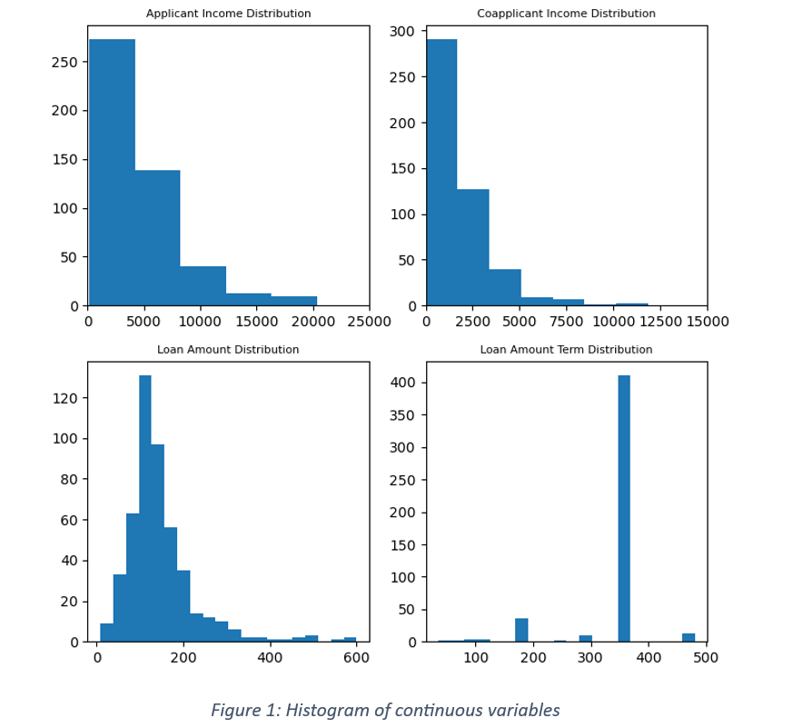
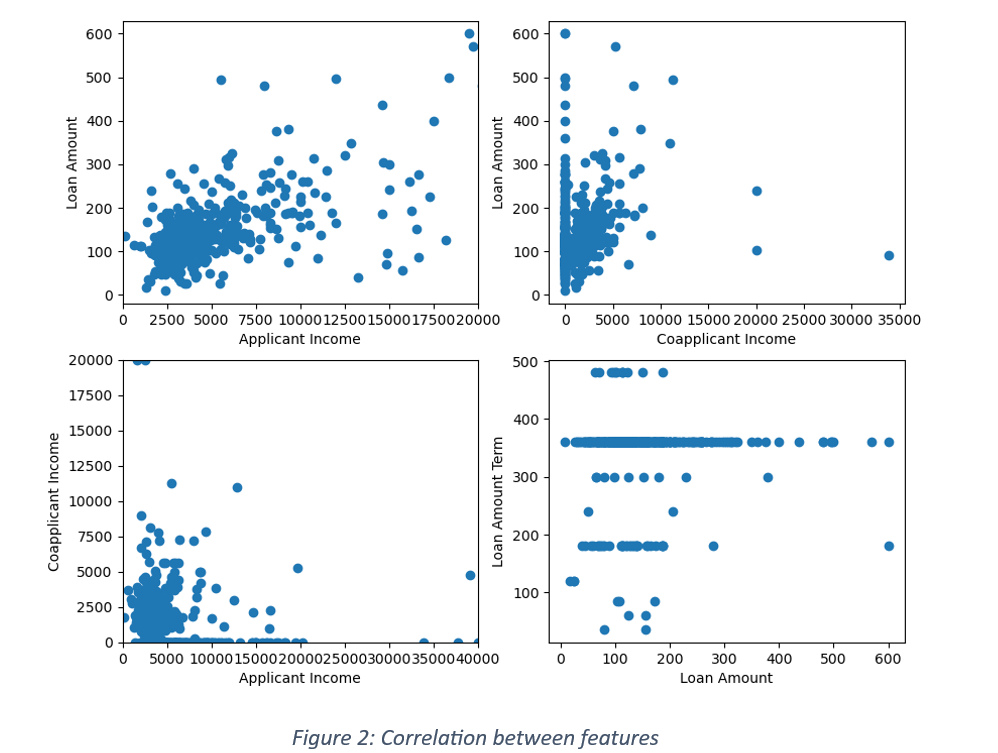
It is a case of binary classification where the response is either ‘Yes’ or ‘No’. An imbalance in the distribution of responses can influence the model’s training process. For instance, if the data has 70% positive responses, there is a higher chance of predicting more approvals than rejections and misclassifying the rejected loans as approved loan applications. The issue of imbalance in the target variable can be handled by distributing a fixed proportion of positive and negative labels between train and test data. The data is further checked for any null values. There were no nulls in the current data. Figure 1 shows distribution of continuous variables and Figure 2 is the scatter plot between features. The applicant income distribution shows most of the applicants falling in less than 10000 income brackets. The income of majority of co-applicants is lower than 5000. There is a weak correlation between applicant income and loan amount and a small shift in the range of borrowed loans with the increase in applicant’s income. Negligible correlation between co-applicant’s income and loan amount shows that the co-applicant’s financial condition is not associated with borrowed loans.
The input variables were segregated into categorical and quantitative variables. The categorical variables were encoded by applying label encoder and one Hot encoder. While any one of them can be used in encoding data, each has its pros and cons. Label encoder encodes categories into integers and one hot encoder encodes into a binary format. It is recommended that Label encoder should be used when the number of classes is limited to 2. For more than 2 classes, integer coding can create unintentional ordinal relationship between categories. For the current data, label coding was used for variables with binary classification viz. gender, marital status, dependents, education, self -employed, property area and target variable. One hot encoding was used for encoding the remaining categorical variables with more than 2 classes.
Feature Engineering
The quantitative variables were subjected to feature engineering. New columns like ratio of loan amount to applicant income, ratio of loan amount to sum of applicant income and co-applicant income were created. All the quantitative variables were normalized. The main reason behind normalization was to limit the range of values and reduce the effect of outliers on machine learning models and their prediction accuracy. By default, the values were transformed into a range between 0 and 1.
Model Building
The pre-processed data was split into train and test with 70% train and 30% test data. There are many classification models like Logistic Regression, gradient boosting classifier, Decision Tree classifier or Random Forest. For the current data, both Logistic Regression and Gradient boosting classifiers like XGBoost were used for model building.
Model training using XGBoost classifier
Hyperparameter tuning was used to minimise the loss function and increase the model accuracy. The chosen hyperparameters were maximum depth, fraction of training samples to train each tree, fraction of features used to train each tree, number of estimators and the learning rate. Grid Search Cross Validation is used to fine tune the hyperparameter values and a 3-fold cross validation is applied. For two class classification, the objective of XGB classifier is binary:logistic and the evaluation metric used for parameter selection is ‘Area Under Curve (AUC)’. Higher the AUC, better the model performance in distinguishing between classes. The parameter values, generating the highest AUC score, are selected and fitted on the train data. The trained model is used to predict probabilities for train and test data.
Model Evaluation
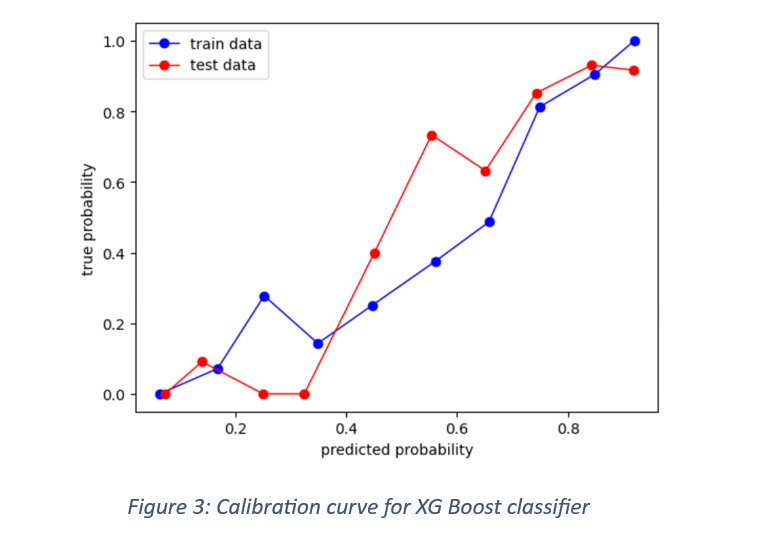
One of the ways of testing a model’s ability to correctly classify the labelled responses is with calibration curve. The curve compares the predicted probabilities with the true frequencies. The calibration curve for train and test data is shown in Figure 3.
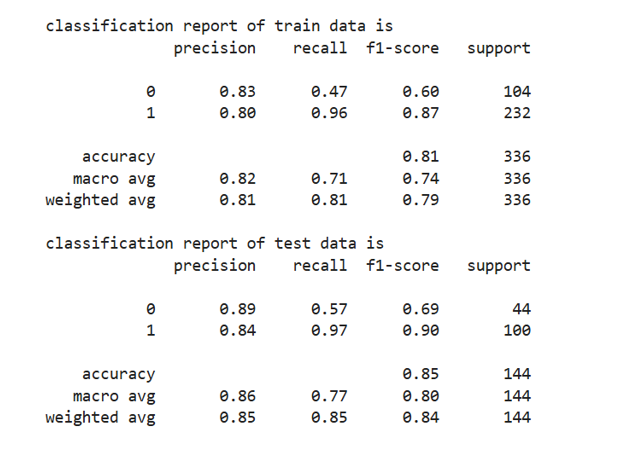
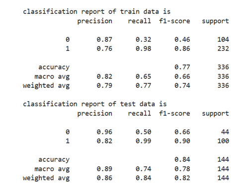
The performance metrics used for model evaluation are: Accuracy score, confusion matrix, precision score, recall score, F1 score and ROC-AUC score. The table shows the classification report for model evaluation on train as well as test data.
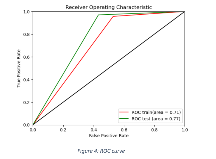
ROC curve was plotted between false positive rate and true positive rates for train and test data, as shown in Figure 4.
Model training using Logistic Regression
The model is trained by applying Grid Search CV to fine tune the hyperparameters of Logistic Regression method. The chosen parameters are the inverse of regularisation strength (C)and elastic net mixing parameter (L1_ratio). The penalty chosen for the model is ‘elastic net’ and the solver is ‘saga’. The model is evaluated, given a range of values of ‘C’ and ‘L1_ratio’ and the best values are selected from the grid. The Logistic Regression, using the best parameter values, is fitted on the train data. The fitted model is finally used to predict for train and test data.
Model evaluation: The classification report is shown here
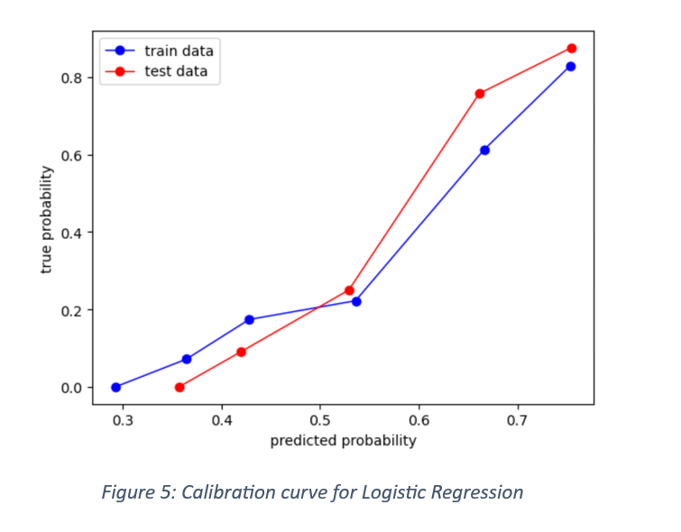
It is observed that the precision and recall of XG Boost classifier are slightly better than those of Logistic Regression for negative labels. The calibration curve showing predicted probabilities against true probabilities are shown in Figure 5.
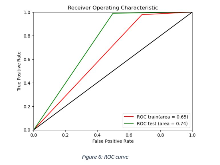
ROC AUC curve for train and test data is shown in Figure 6.
Model Comparison
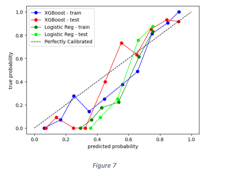
As mentioned earlier, there is not much difference in precision and recall values of Logistic Regression and XG Boost classifier in the context of positive labels. XG Boost, however, performs slightly better in the classification of negative labels. Figure 7 shows calibration curves of both the models applied on train and test data.
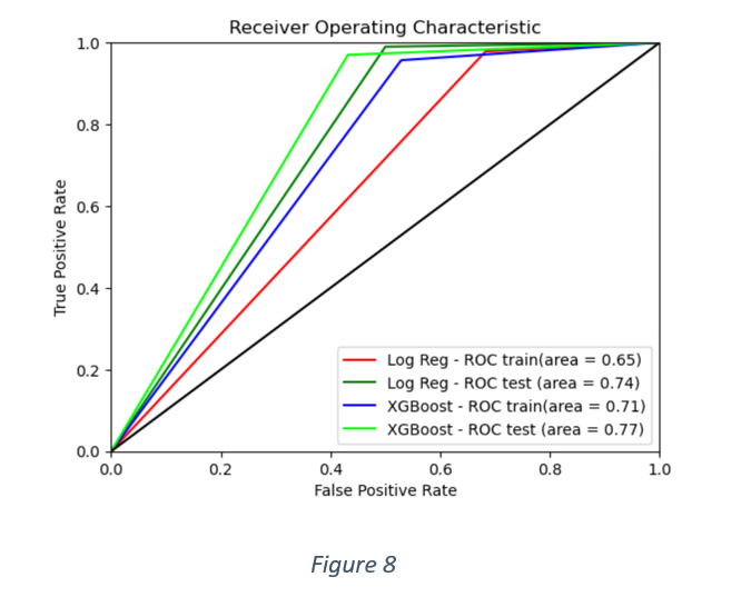
A better picture of relative model performance can be gauged from AUC scores, as shown in Figure 8. The overall performance of XG Boost classifier is better than Logistic Regression.
Model insights
The model accuracy of XG Boost classifier was improved by observing ROC AUC score for different combinations of hyper parameters like fraction of features to train each tree, learning rate, maximum depth, number of estimators and fraction of training samples to train each tree. The combination with the maximum AUC score was used in fitting the model to the train data and predicting loan approvals of the test data. There is a trade-off between the learning rate and number of estimators. The higher learning rate of 0.3 was balanced with only 50 estimators.
It is observed that the ability of the chosen model to discriminate between classes improves on test data. The accuracy score, precision, recall, F1 and ROC-AUC scores of test data are higher than those of train data. However, the caveat is that the precision, recall and F1 scores are assumed around the model’s ability to correctly classify true positives. But the confusion matrices show higher number of false positives than true negatives. Hence, the recall scores for negative labels (XG Boost) are 0.47 for train data and 0.57 for test data. Overall, the model performance is better for the test data than train data. It is likely that an imbalanced distribution of positives and negatives builds a model that misclassifies many loan application rejections as approvals.
Feature importance
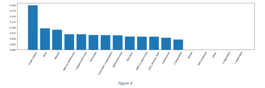
The above plot shows that the most important feature in loan application assessment is credit history. The least important features are gender, whether the applicant is self-employed, whether the applicant has 0 to 1 dependent and whether the property is in urban area or not. Other important features are marital status, applicant and co-applicant income, debt to applicant and total income ratios, semi-urban and rural area of the property, more than 3 dependents, loan amount and loan term. It may be inferred that an applicant’s credit history, property location, marital status, debt to total income and number of dependents should be prioritised in loan approval decisions.