Introduction
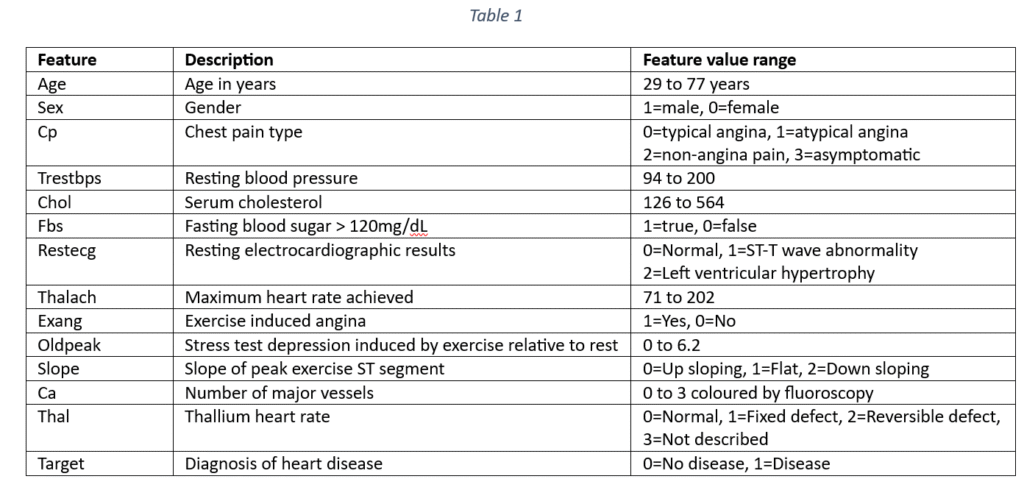
The dataset contains 133 samples for predicting the occurrence of heart disease. Each sample has 13 features that can be used to predict cardiac failure. The features include demographic details like age and sex and clinical indicators. The cardio-vascular disease indicators are: Type of chest pain, Blood pressure, Cholesterol, fasting blood sugar, resting electrocardiographic results, Maximum heart rate achieved, Exercise induced angina, Old peak, Slope, Number of major vessels coloured by fluoroscopy and Thalassemia. The target variable is the occurrence or non-occurrence of heart disease. The features are explained in Table 1.
The objective of data analysis is to predict the prevalence of heart disease from a set of factors represented as features in the data set. The objective also includes an identification of the most important factors for predicting the heart disease.
Data pre-processing
First, the data is checked for any missing or null values. For any missing value, the data column is identified as categorical or quantitative. In case of quantitative columns, the median of column values fills the missing values. In case of categorical data, the mode or the most frequently occurring category fills the missing data. The current data does not have any missing values.
Next, the categorical variables are identified and converted into datatype ‘category’. The categorical data is encoded by using One-Hot encoding. One-Hot encoding encodes the categorical variables with more than two categories. The category names are assigned to the categories of each qualitative variable. The implementation of One-Hot encoding transforms each qualitative variable into a set of columns where each column represents the presence or the absence of a class/category of the variable. For instance, ‘Chest pain type’ is a categorical variable in the original data with four categories represented as ‘0’, ‘1’, ‘2’ and ‘3’. The categories in the numerical form are mapped into category names with string data type.
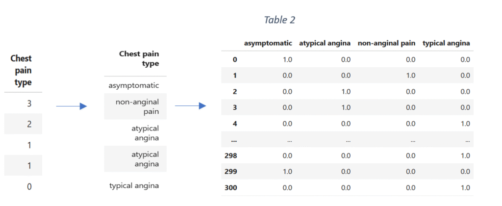
The data is then one hot encoded, converted into a data frame and concatenated with the original data. After transformation, the original column ‘Chest pain type’ is dropped. The process of data encoding is repeated for the remaining categorical variables.
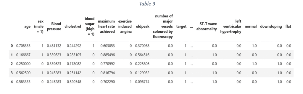
After one hot encoding, the quantitative variables are identified and scaled to a fixed range between 0 and 1. ‘Minmax scaler’ scales the data and is suitable even when the data distribution is not Gaussian. For the given data, variables like age, blood pressure, cholesterol, maximum heart rate achieved, old peak and major vessels coloured by fluoroscopy are scaled using ‘Minmax scaler’. The final dataset in shown in Table 3.
Exploratory data analysis
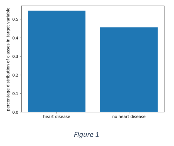
Figure 1 shows that the distribution of target variable is not perfectly balanced. More than 50% of the samples have positive labels. However, the data is not entirely imbalanced as the overall distribution is 55% and 45%.
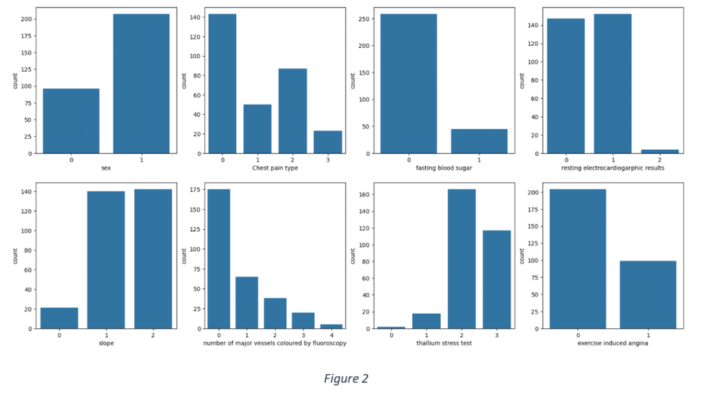
Figure 2 shows the frequency distribution of categorical data. Most of the use cases are males, have fasting blood sugar within the recommended range, have either normal or ST-T wave abnormality from resting electrocardiographic results, reversible defect from thallium stress test results and typical angina or non-angina pain.
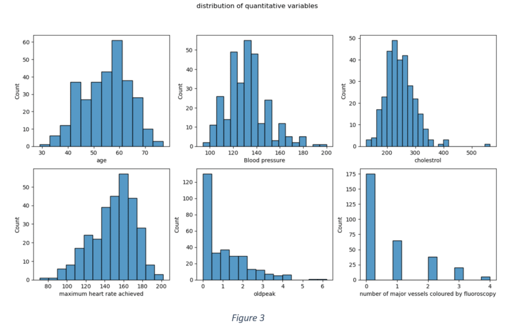
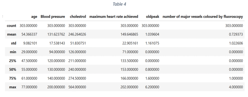
Figure 3 shows the data distribution of quantitative features. None of the quantitative variables has an ideal Gaussian distribution. The distribution of ‘Age’ is slightly Gaussian with mean = 0.53. ‘Blood pressure’ and ‘Cholesterol’ are slightly skewed towards left with means < 0.5 (0.36 and 0.27 respectively). This shows that 75% of the use cases have blood pressure levels lower than 140 and cholesterol less than 274. The Maximum heart rate distribution is skewed towards right with mean rate = 150 and maximum = 202. Most the use cases have old peak values lower than 1.6 and the maximum recorded old peak is 6.2. The Number of major vessels coloured by fluoroscopy is fewer than 1 for majority of the data samples. The descriptive statistics of quantitative features is shown in Table 4.
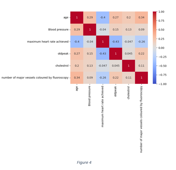
Apart from the data distribution of each quantitative variable, the correlation matrix in Figure 4 shows that nearly all the quantitative features are weakly correlated. The highest correlation is -0.43 between old peak and maximum heart rate achieved. The correlation between maximum heart rate and age is -0.43. Hence, the association of each feature with the target variable can be analysed independent of other features.
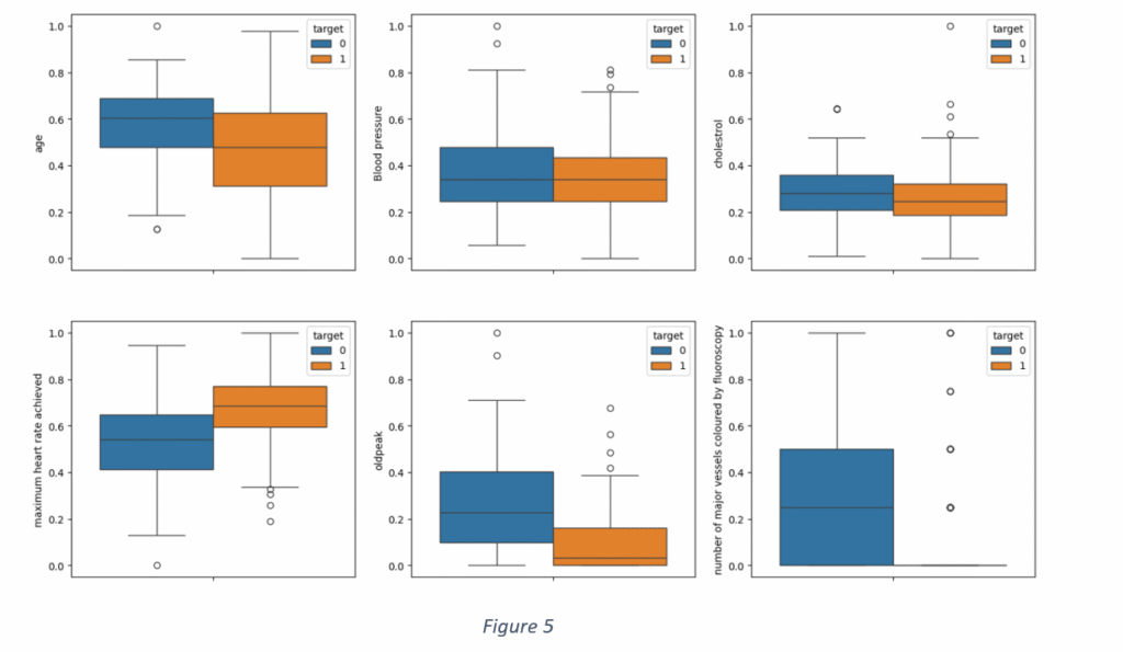
A distribution of the quantitative features for each class of target variables is shown in Figure 5. It is observed than blood pressure and cholesterol levels are not suitable indicators of heart disease, given a large overlap between positive and negative labels of the target variable. A distribution of ‘Maximum heart rate achieved’ shows that the maximum heart rate, for nearly 75% of the cases without heart disease, was less than 155. On the other hand, the maximum heart rate was beyond 150 for 75% of the samples with the heart disease. Similarly, there is a small overlap in ‘old peak’ values with most of the old peak values less than 1 for the cases having heart disease and more than 1 for cases with no heart disease. The distribution of ‘Major vessels coloured by fluoroscopy’ proves that the major vessels of the patients of any cardiovascular disease are blocked and cannot be coloured by fluoroscopy. However, there are few outliers where the major vessels are coloured even in heart patients. It is not difficult to ascertain if age contributes to heart diseases, given small size of 133 samples and an overlap between occurrence and non-occurrence of heart disease.
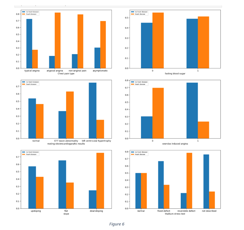
The relationship between categorical data and the target variable was gauged by observing the distribution of different categories of each categorical feature against the target, as shown in Figure 6. The chest pain distribution shows that 60% to 80% each of asymptomatic, atypical angina and non-anginal pain samples had heart disease. Similarly, most of the cases with symptoms of down sloping, reversible defect in thalassemia and the absence of exercise induced angina had no heart diseases.
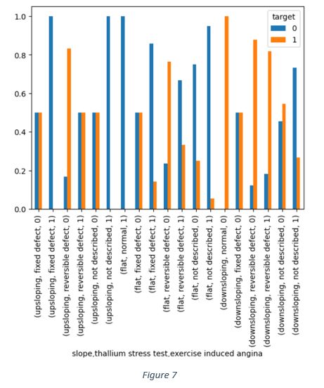
The combined impact of slope, thallium stress test and exercise induced angina in Figure 7 shows that the reversible defect in thallium heart rate is one of the dominant factors associated with occurrence of heart disease.
Feature selection
Given a weak correlation among quantitative variable, the distribution of each quantitative variable against target variable was analysed independently. It is observed from Figure 5 shows that ‘Blood pressure’ and ‘Cholesterol’ are not suitable indictors, given a large overlap between positive and negative labels of target variable. The ‘Age’ distribution shows 75% of cases of heart disease with age less than 65 and 75% of cases without heart disease falling the age group 20 to 70. Age, alone, may not be a reliable indicator.
Figure 6 shows that nearly 55% of people, with blood sugar levels below 120mg/dL, have heart diseases. Out of those with higher blood sugar levels, nearly 48% do not have heart disease. It is, therefore, difficult to infer any strong association between blood sugar and prevalence of heart disease. Similarly, there are 50% of cases of heart diseases under normal results in thallium stress test, making it a weak indicator of any heart disease. There is also a little difference between the percentage of cases with and without heart disease under up sloping or normal conditions in resting electrocardiographic results. Figure 7 also shows that the reversible defect in thallium stress test and the down sloping condition are dominant factors associated with the prevalence of heart disease.
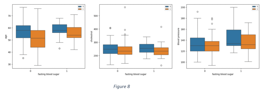
Figure 8 shows distribution of some quantitative variables against ‘Blood sugar’ for positive and negative cases of heart disease. It is observed that there are overlaps between ‘Age’ and ‘Blood sugar’, ‘Age’ and ‘Cholesterol and ‘Age’ and ‘Blood pressure’ notwithstanding the prevalence of heart disease.
After analysing the relationships among the features and between features and target variable, it was inferred that ‘Age’, ‘Cholesterol’, ‘Sex’, ‘Blood sugar’, may have weak association with the target variable. Hence, the features selected for model building are:
‘Typical angina’, ‘Reversible defect’, ‘Number of major vessels coloured by fluoroscopy’, ‘Old peak’,’ Maximum heart rate achieved’, ‘Non-Angina pain’, ‘Atypical angina’, ‘Asymptomatic’, ‘Left ventricular hypertrophy’, ‘Exercise induced angina’, ‘Down sloping’, ‘Not described’, ‘Flat’, ‘Up sloping’, ‘Fixed defect’, ‘ST-T wave abnormality’.
Model development
The dataset is split into train and test data. 80% of the data is train. The train data is further subjected to cross validation to select the model with most optimal parameter values. The balance is used to test the model performance.
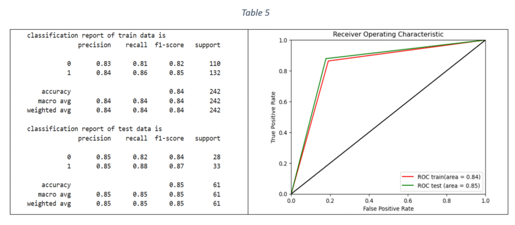
Logistic Regression (LR): Logistic Regression is a binary classification technique. The model is trained by using Stratified-K-fold cross validation and tuning the hyper-parameters with Grid Search Cross validation. Stratified-K-fold cross validation is effective in handling imbalanced datasets by ensuring that the proportional distribution of classes in every fold is same as in the original dataset. The parameters used for model tuning are penalty, class weight, maximum number of iterations and inverse of regularisation strength. The metric used to select the best parameters is F1 score. F1 score is the harmonic mean of recall and precision and can handle any imbalance in the target variable. The selected parameters with the highest F1 score were used to fit the final model on the train data. The classification report and ROC-AUC graph are shown in Table 5.
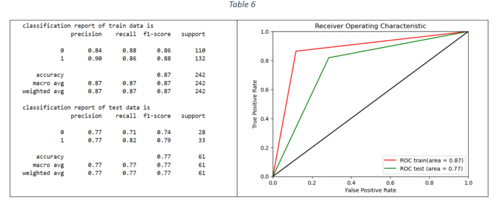
Decision Tree (DT) classifier: Decision tree classifier is suitable for binary classification. The decision tree is used to predict the target value by splitting the data based on one feature at a time. The classifier parameters for hyper-parameter tuning are criterion, maximum depth, minimum number of samples required to split an internal node, maximum number of features to consider for the best split, minimum number of samples per leaf node and class weight. Based on F1 score, the best parameters are selected for training the DT model on train data. The classification report and ROC-AUC are shown in Table 6.
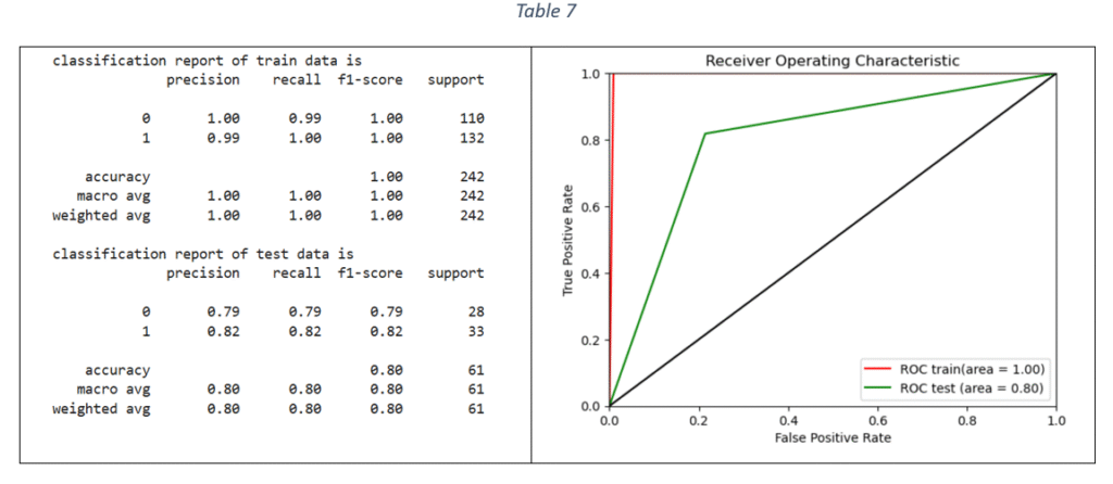
Random Forest (RF) classifier: The Random Forest uses multiple decision trees on various sub-samples of the dataset and uses averaging to predict the target values. The hypermeters for tuning the model and selecting the best Random Forest parameter values are: number of estimators, criterion, maximum depth, minimum number of samples for each internal node, maximum features to consider the best split and class weight. The optimal parameter values are selected with hyper-parameter tuning and the final model is trained on the train data (using the most important features). The classification report and ROC-AUC graph are shown in Table 7.
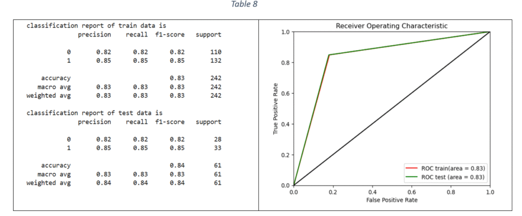
Support Vector Machines: Support Vector Machine (SVM) is classification method and is effective when the relationship between features and target variable is complex and non-linear. Grid Seach CV is used to tune the following hyper-parameters: Inverse of regularisation strength, type of kernel, type of kernel coefficient and class weight. The model with the best parameters is fitted on the train data. The classification report and ROC-AUC graph are shown in Table 8.
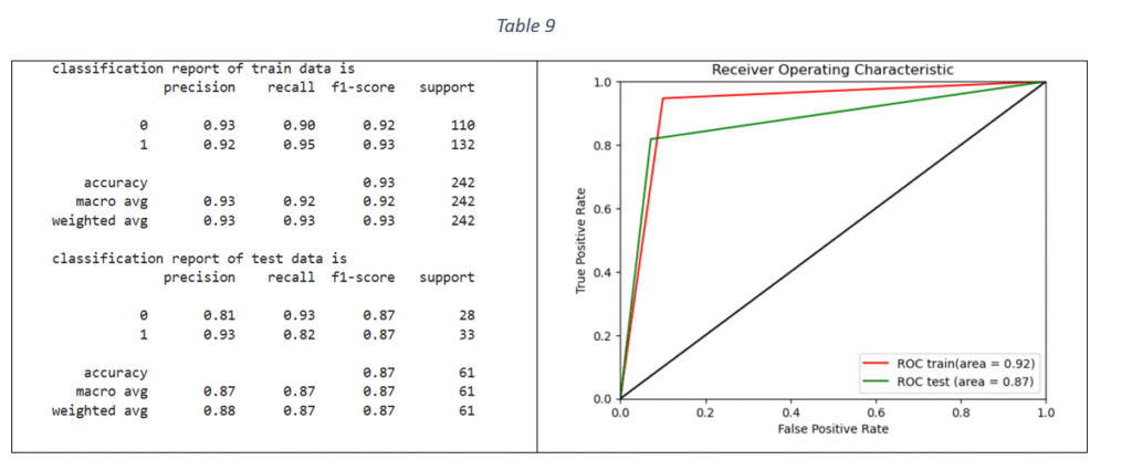
XG Boost Classifier: Extreme Gradient Boosting algorithm is based on sequentially combining multiple decision trees where the classification error in the preceding tree is acknowledged and corrected in the succeeding ones. By applying Grid Search and Stratified-K-fold cross validation, the tuned hyper-parameters are: maximum depth of each decision tree, ratio of samples randomly sampled for each decision tree, fraction of features randomly sampled for each decision tree and considered for splitting at each node, learning rate, number of decision trees required to build the model, L1 regularization and L2 regularization. The classification report and ROC-AUC graph is shown in Table 9.
Model comparison
Table 10 is a comparison of accuracy, recall, precision and F1 score of all the models on test data.
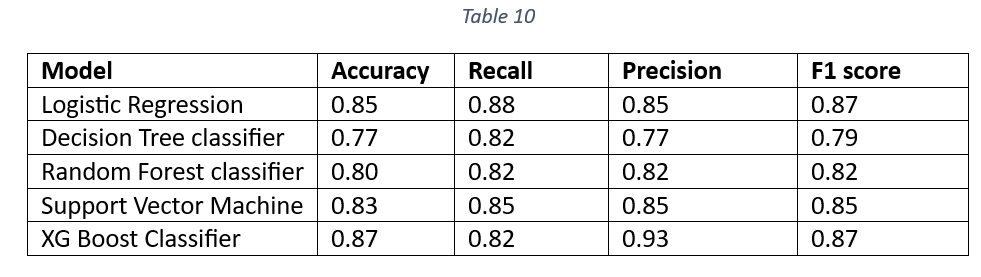
The Accuracy, Precision and F1 values of XG Boost Classifier are the highest. The higher Accuracy and F1 values of XG Boost Classifier make it a suitable candidate for the final model selection. The Decision tree classifier is the worst performer, suggesting that DT classifier cannot be selected as the final model. Figure 9 shows the Area Under the Curve (AUC) curve of all the models. The comparison of AUC curves is done separately for train and test data.
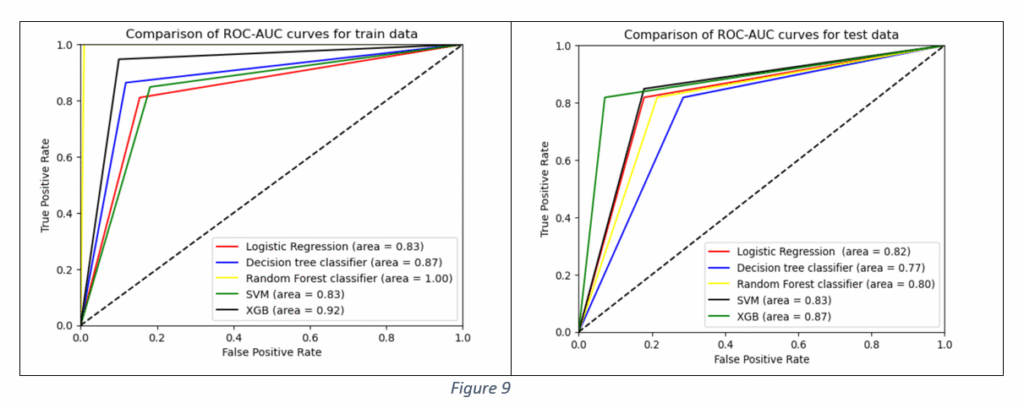
It is observed from Figure 9 that Area Under Curve (AUC) value of Random Forest Classifier is the maximum on train data. However, the performance worsens on test data, indicating the model’s ability to pick up train data patterns with higher accuracy. Decision Tree AUC is better than Logistic Regression and SVM classifiers but the performance is the worst on test data among all the models, proving that the tree structure can get altered for any new data. The Decision Tree exhibits the problem of overfitting, as it becomes unstable with slight variations in data. The variations are acute with high dimensional data. The classifier’s performance improves for large sample sizes, fewer features and balanced distribution of classes in categorical data. In the given case, the dataset had only 133 samples and large number of features.
The Random Forest performs better than Decision Tree. However, the values of performance metrics like accuracy, F1 score and ROC-AUC are better on train data than on test data. Although RF is robust to overfitting, it can still overfit if there is noise in the train data. Logistic Regression is suitable for binary classification and performs better with small sample sizes. The Logistic Regression AUC values are nearly the same performance for both train and test data. The XG Boost classifier performance in terms of Accuracy, Precision, Recall, F1 and ROC AUC is better than other machine learning algorithms. Hence, XG Boost classifier is selected as the final model.
Model deployment
Creating web application: A web application framework named Flask was used for developing an interface that accepts patient input details and generating response for heart disease prediction. First, the trained model is saved as pickle file named ‘model.pkl’. Next, an application file named ‘app.py’ is created in python. The file is the core of web application that responds to user requests based on the type of request. The Flask app is initialised and two functions are created. The first function is to display the content of HTML page of web app. The second function ‘POST’ is used to retrieve information from HTML file, feed the data to the trained model and send the prediction back to the HTML file to display the result. The third file is HTML file named ‘index.html’ stored in a ‘Templates’ folder. The HTML file consists of HTML code for creating input fields. The value entered in each input field, representing an independent variable, is fed to the model by using the function ‘request.form.get’ in the ‘app.py’ file. The independent variables used for this web app included only the most important features as explained in ‘Feature selection’ section.
Deployment of web app: Following are the files created for web app deployment:
- model.pkl
- app.py
- Templates/index.html
- Procfile
- Requirements.txt
All the files are uploaded on a Git Hub repository. A new app named ‘cvd-prediction’ is created in Heroku (web application hosting platform) and is connected to the Git repository. All the Git files are pushed to Heroku. The web app gets activated and can be accessed at the following link:
https://cvd-prediction-cd2be672a63c.herokuapp.com
Future improvements
It is observed that even the best model cannot predict more than 87% of the labelled responses accurately. The model performance can be improved by increasing the number of data samples. It is unlikely that a new advanced algorithm can improve the performance. The ambiguity in relationships between the prevalence of heart disease and factors like ‘Cholesterol’, ‘Blood pressure’, ‘Blood sugar’ and ‘Age’ can be overcome by applying stratifying sampling. The collection of a large number of samples separately for different age groups and an equal distribution of samples between the two classes of gender can provide a clearer picture of the association of ‘Age’ and ‘Sex’ with heart disease prediction. A large sample size may also significantly alter the strength of association between ‘Blood sugar’, ‘Old peak’, ‘Exercise induced angina’ and ‘Slope’ and the heart disease prediction.